
# Algorithm & Datastructures
My knowledge compilation of algorithm & datastructures.
# Referenced Sites
- Harvard CS50 (opens new window)
- Samsung SW Expert Academy (opens new window)
- Master the Coding Interview (opens new window)


알고리즘 복잡도
알고리즘은 효율적이여야한다. 설계 자원분석 효율성 제시
공간적 효율성 : 메모리 공간
시간적 효율성 : 연산 시간
효율성의 반대말 = 복잡도
시간적 복잡도로 알고리즘의 효율성을 평가할 수 있다.
Big O : 복잡도의 점근적 상한. 최고차항만 고려.
Big Omega : 점근적 하한. 최고차항만 계수 없이 고려
Theta = O 와 Omega가 같은경우.
효율적인 알고리즘은 슈퍼컴퓨터보다 더큰가치가 있다.
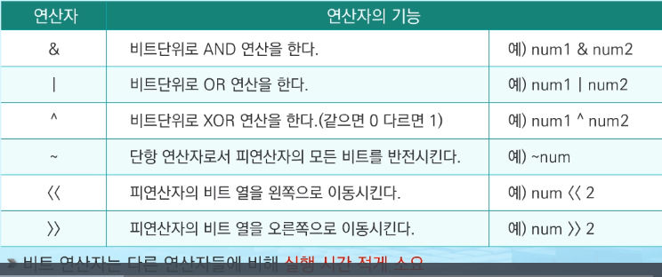
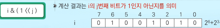
비트연산자

완전검색기법
가능한 모든 경우들을 나열해보고 확인
brute force, generate and test라고도 불린다. 빠른시간안에 알고리즘 설게가능. 대부분의 문제에 적용가능.
순차검색 : 첫번째 자료부터 비교하면서 진행. 존재하지 않는경우가 최악의 경우.
문제의 크기가 커지면 시간복잡도가 매우 크게 증가.
그리디 기법이나 동적계획법으로 더 효율적인 알고리즘을 찾을수있다.
문제를 풀때 완전검색으로 해답도출후 성능개선을 위해 다른 알고리즘을 사용할수있다.
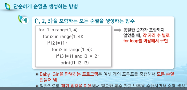
베이비진의 경우 모둔 순열을 나열하고 앞세자리와 뒤세자리를 잘라서 베이비진 테스트를 해볼수있다.
중복을 제거 할 수 있따면 시간을 아낄수있다.
조합적 문제
순열, 조합, 부분집합과 같은 조합적 문제들과 완전검색은 관련돼있다.
완전검색은 조합적문제에 대한 brute force 이다.
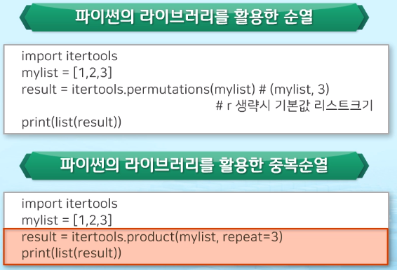
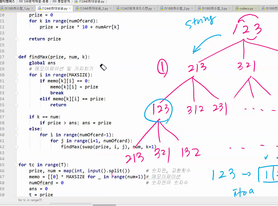
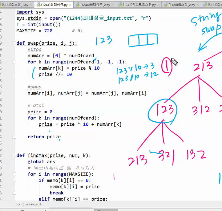
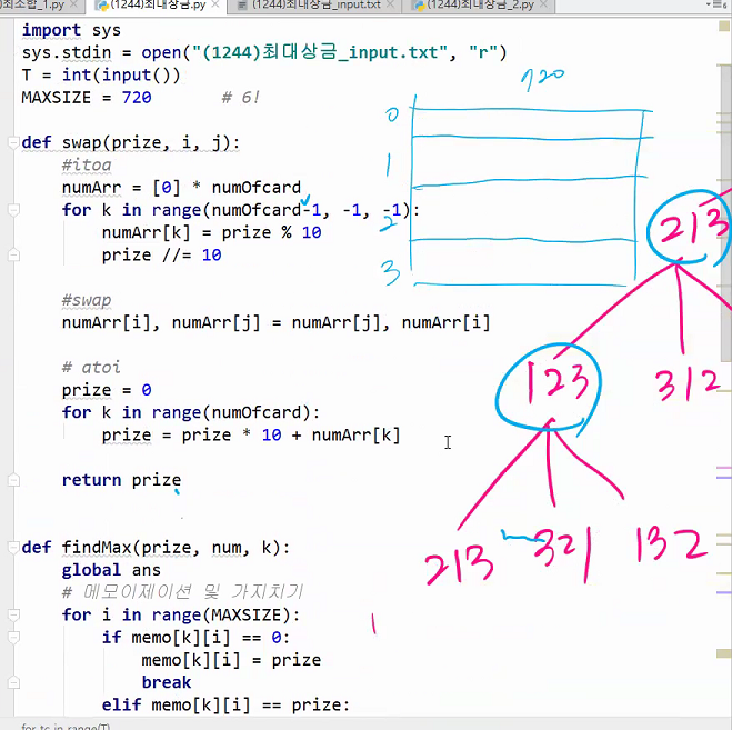
순열
한줄로 나열. n개 중 r를 선택. nPr로 표현된다. nPn은 n!과 동일하다
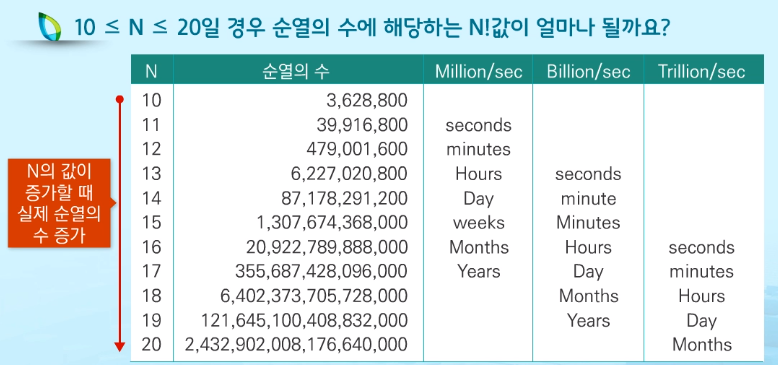
기하급수적으로 실행시간이 증가한다. 현실적으로 완전검색은 하기 힘들어진다.
사전식 순서 : 요소들이 오름차순으로 나열된 형태가 시작하는 순열
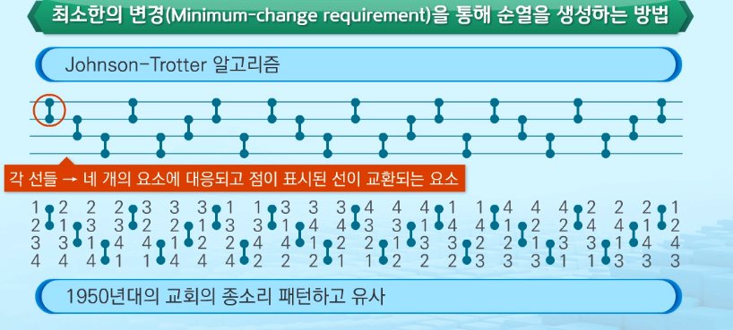
최소 변경을 통한 방법 : 각각의 순열들은 이전의 상태에서 두개의 요소를 교환하여 생성.
- Johnson-Trotter 알고리즘.
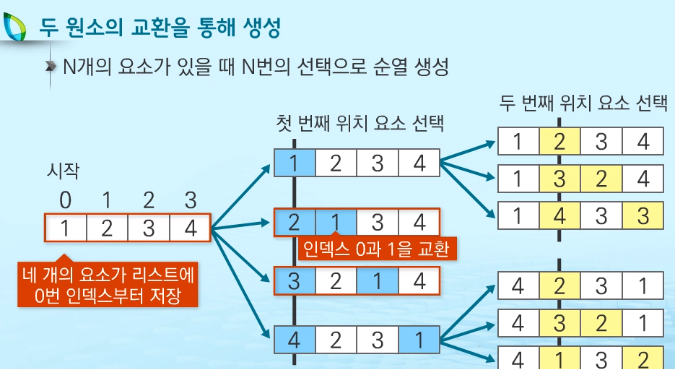
원소교환을 통한 방법 : 최소교환은 아니지만 자주 사용된다.
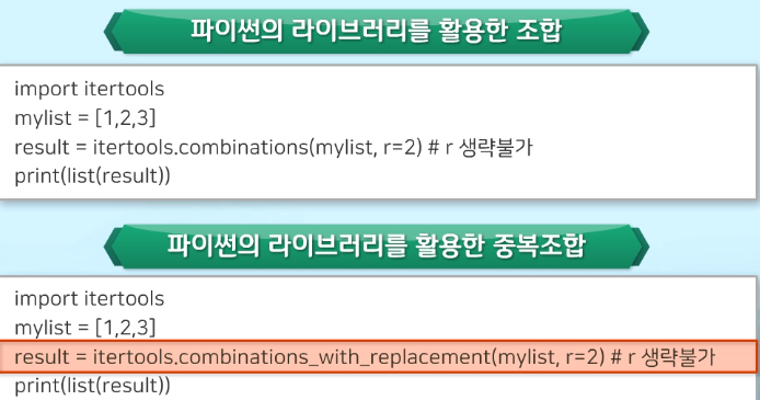
파이썬의 라이브러리를 이용한 방법 :
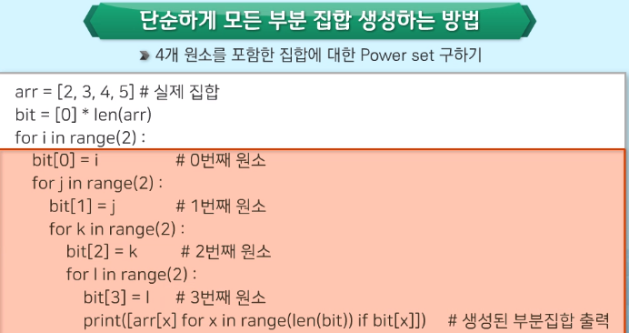
부분집합
Knapsack Problem

탐욕기법과 동적에서 배우게된다.
단순하게 모든 부분집합생성하는 방법

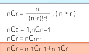
조합
서로다른 n개의 원소중 r개를 순서없이 골라낸것. nCr
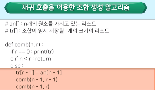
- 라이브러리를 활용한 조합과 중복조합
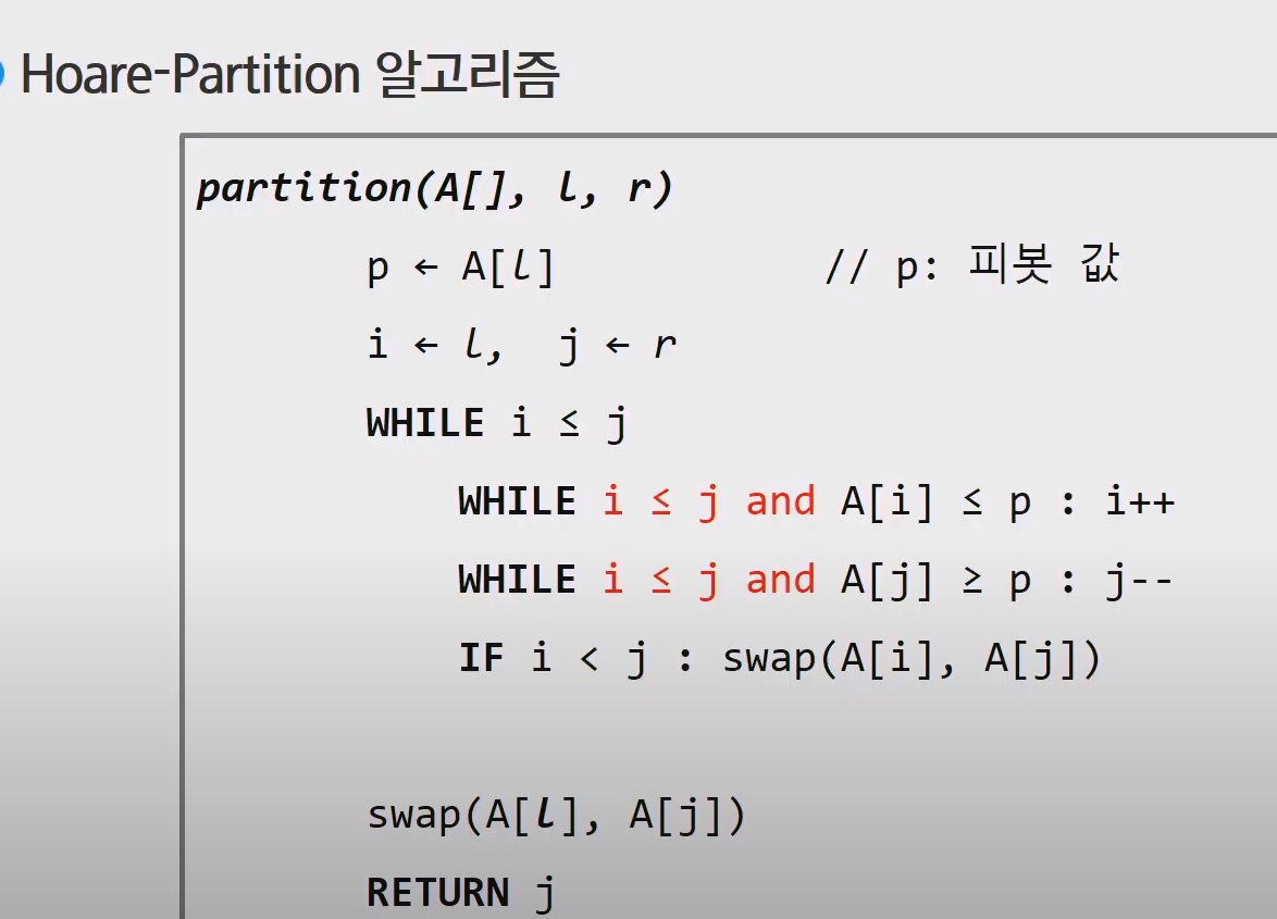

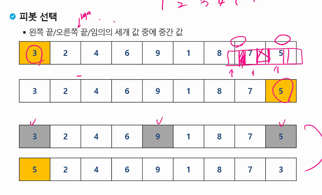
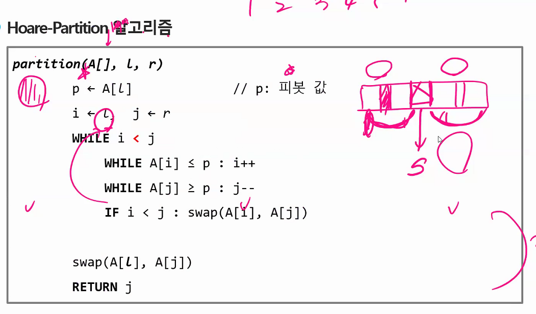
중간값으로 해야 최악을 벗어날수있다. 보통은 편하니까 제일 왼쪽꺼하는데 재수없게 1이라던가 그런거 걸리면 n^2 다해야된다.

# Datastructures
# Big O
# Arrays
# Hash Tables
# Linked Lists
# Stacks
- What is a stack?
- Like a stack of plates. It is 'Last In First Out'.
- Usually programming languages are made with stacks in mind.
- ctrl+z, go back page in internet are all examples of stacks.
- big O is (n)
- pop : remove the last item
- push : add a item
- peek : view the last item
- How to implement
- Using arrays
- Using Linked Lists
- How it works - Calculator
- prefix, infix, postfix notation : placement of operators and operands. Infix is commonly used but computers use postfix notation to calculate.
- How to change from infix to postfix
Prepare stack for operators.
Read token
If token is operand(numbers) → print
if token is operator → compare with last item in stack → if no operator in stack : push. if token's priority is higher : push, else :pop until token's operator is higher, then push
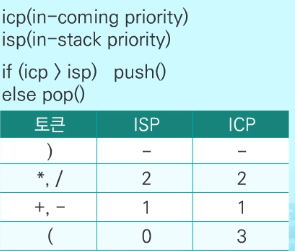
if token is right bracket
): pop and print operator in stack UNTIL(left bracket is popped. bracket is not printedRepeat until nothing to read from infix
Finally pop everything from operator stack.
(left bracket outside the stack has highest priority.)right bracket inside stack has lowest priority.
- How to calculate using postfix
- Prepare stack for operands.
- Push to stack if operands
- If operator → pop from stack twice → calculate.
first pop - operator - secondpop→ push value back to stack - If finished : pop from stack
# Queues
- What is a queue
- Like a roller coaster queue, its 'First In First Out'.
- Examples are, uber, ticket buying, printer.
- Front means the first among items. Rear means last item saved.
- big O is (n)
- enQueue() : add item. check full. Add 1 to rear and place new item at the new rear position
- deQueue() : remove first item. check empty. Add 1 to front and return new item at the front position
- createQueue() : Makes empty queue
- isEmpty() : check if queue is empty. front == rear == -1
- isFull() : check if queue is full. rear == n-1
- peek() : check whats the first item to come out. checkempty then return Q[front+1]
- How to implement
Using arrays : Not a good idea. Because you need to shift everything when the first item is removed.
Linked Lists :
createQueue() : Empty queue created, front = rear = -1, size=1
enQueue() : front = -1 , rear = 0 /
enQueue() : front = -1 , rear = 1
deQueue() : front = 0, rear = 1 /
enQueue() : front = 0, rear =2
deQueue() : front = 1, rear =2
deQueue() : front = rear = 2
we know when front=rear queue is empty
States of Queue
- Initial : front = rear = -1
- Empty : front = rear
- Full : rear = n - 1
- Arrays vs Stacks vs Queues
- Stacks and Queues are different in that the direction of item being removed.
- Array can have random access to items inside
- Stacks and Queues have limited access. Having a limited access is actually a benefit
- Circular queue
- initial state : front = rear = 0
- when front or rear reaches n-1, index reset to 0.
- front is always left empty
- createQueue() : n=1, front = end =0
- isEmpty(), : front = rear
- isFull() : (rear +1)%n =front
- enQueue() : check if Full. rear ← (rear+1)%n; cQ(rear)=item
- deQueue(): check if empty; front←(front +1)%n ; return cQ[front]
# Trees
What is a tree
- 1:N relationship. It is non-linear.
- Edge : the relation. Node : the items.
- Height : height of root is either 0 or 1. Height of tree equals to the highest node's height.
Binary Trees
- Special kind of tree where all the nodes have maximum of two children.
- If the height is
H, minimum number of nodes isH+1and maximum is2^h+1 - 1 - Most commonly used in programming
- There are three types of binary trees
- Full binary tree: Every node is full and has
2^h+1 - 1of nodes - Complete binary tree : When height is h, number of nodes are $2^h <= n < 2^h*2^1 -1$. and no node number is empty between 1 and n.
- Skewed binary tree : One sided tree (no value for programming, rather use a list)
- Full binary tree: Every node is full and has
Traversal
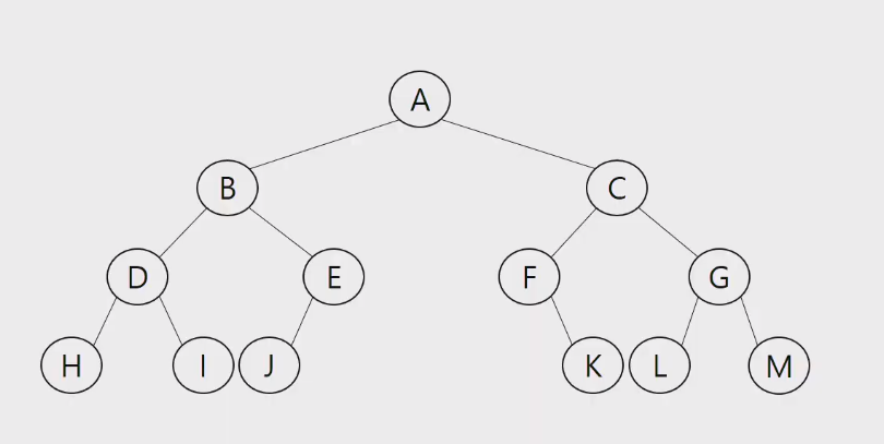
Preorder: A B D H I E J C F K G L M
Inorder : H D I B J E A F K C L G M
Postorder : H I D J E B K F L M G C A
- Visiting every node without duplicates.
- Because trees are not linear, we cannot know the order. That's why we can decide from these three
- Preorder : V L R (root left right)
- Inorder : L V R
- Postorder : L R V
How to implement
- Using Lists
- Every node is given a number, starting from 1 given to root
- Level N nodes have numbers given from 2^n to 2^(n+1) - 1
- Node i's parent node is i//2
- Node i's left-child is 2*i
- Node i's right-child is 2*i+1
- For tree with height H, you need a list with length of 2^H. list[0] is not used.
- You can see this uses much more memory than needed (especially for skewed trees).
- Linked lists can be used to improve efficiency.
- Using Lists
Binary Search Tree
- Datatype used for efficient searching
- Every item has different key
- left subtree's key < parent's key < right subtree's key
- When tranversed in inorder, it returns ascending ordered keys.
- searching's O(h) is h. Average is O(log n). Worst case O(n)
Heap
- Datatype used to get the maximum or minimum value.
- By definition every key must be different.
- When adding item, temporarily add it to the next place. Then swap it with parent until size relationship is ok.
- When deleting item, can only delete the root item. Therefore, you are able to implement 우선순위 queue with heap.
- First delete the root node. Next, move the 'last' node to the root node. Start swapping between child and parent.
# Graphs
# Algorithm
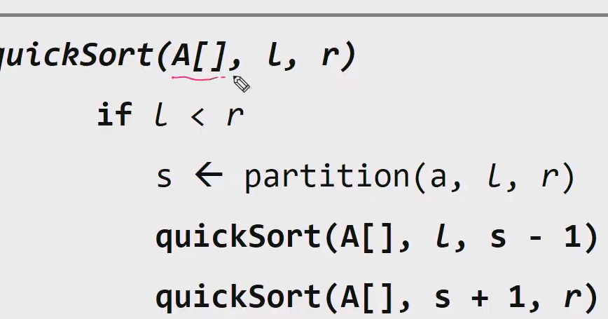
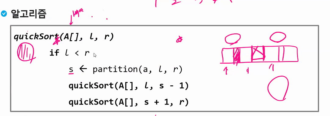
# Sort
# Selection Sort
# Bubble Sort
# Insertion Sort
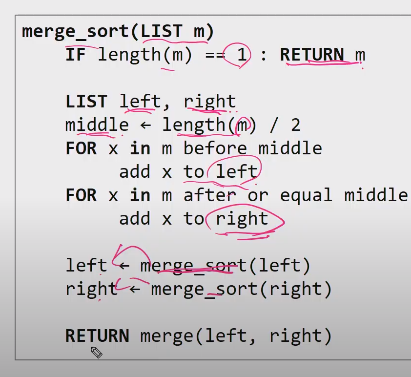
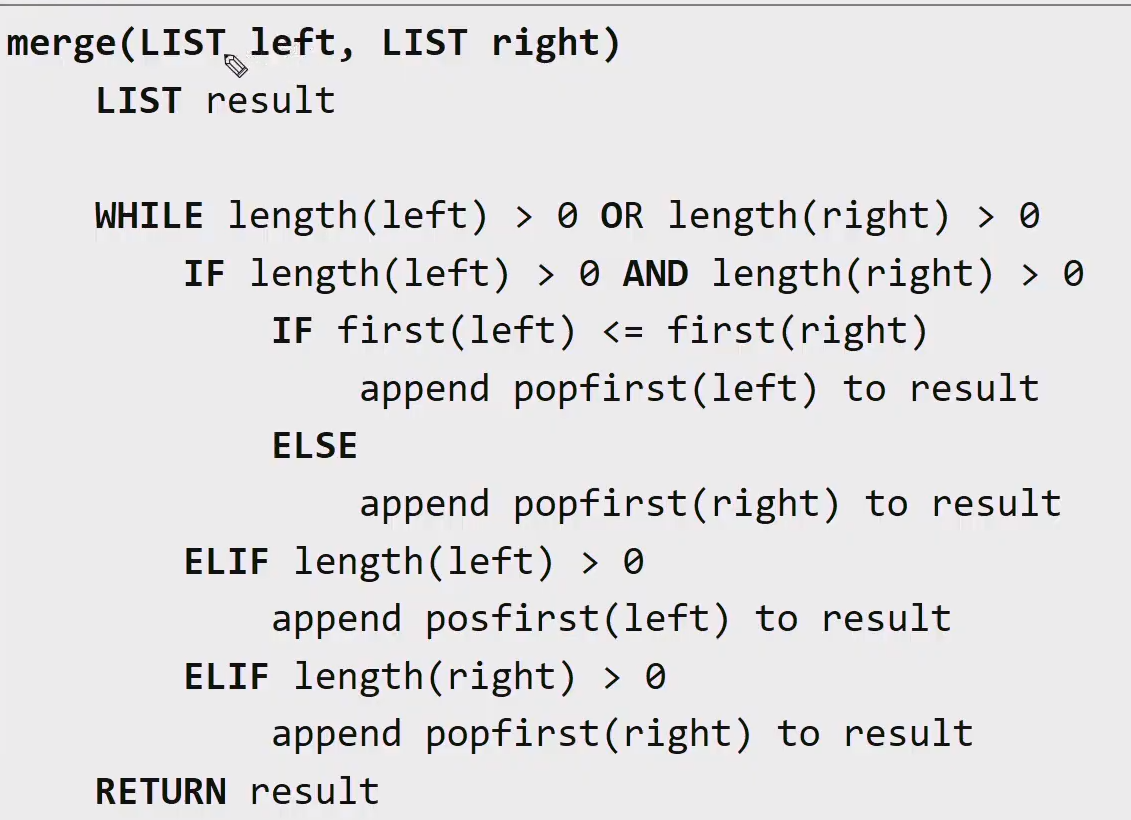
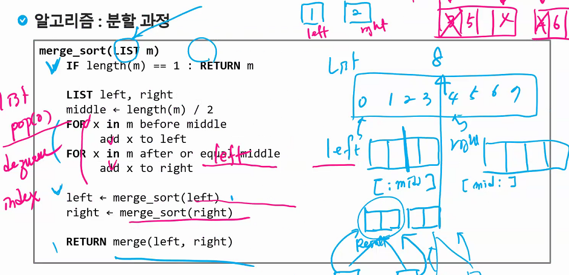
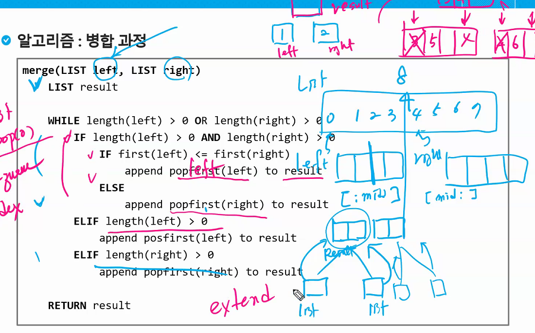
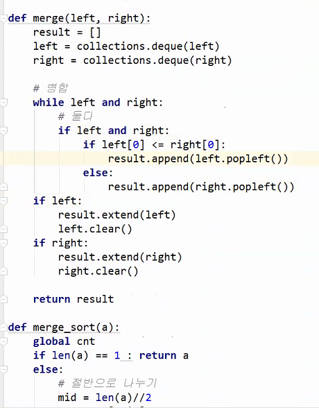
# Merge Sort
# Linear Search
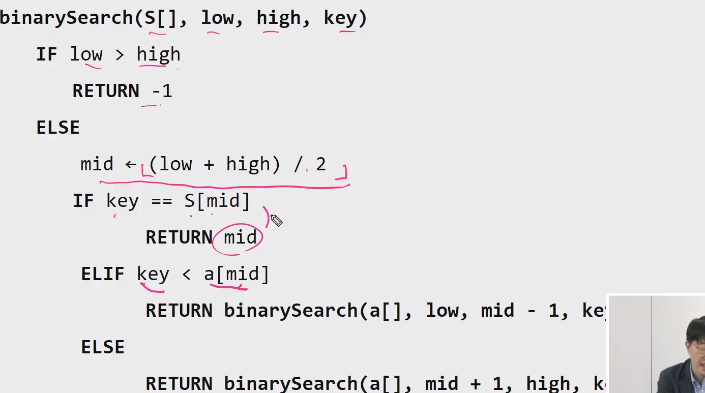
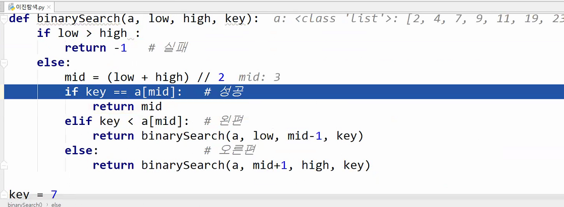
# Binary Search
# Recursion
# DP
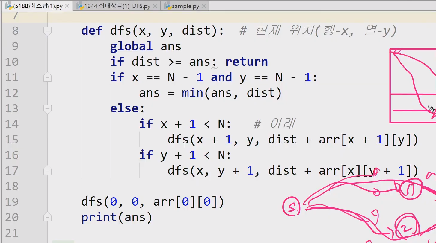
# DFS
- How it works
- Current Location : V, Unvisited Connected Location : W
- Two stacks needed : visited true false stack and last visited push/pop stack
- starting point set as V
- move to W and push V to stack
- set W as V and recall
- IF, there are no W left, pop from stack and set last added V as V again.
- Repeat Process
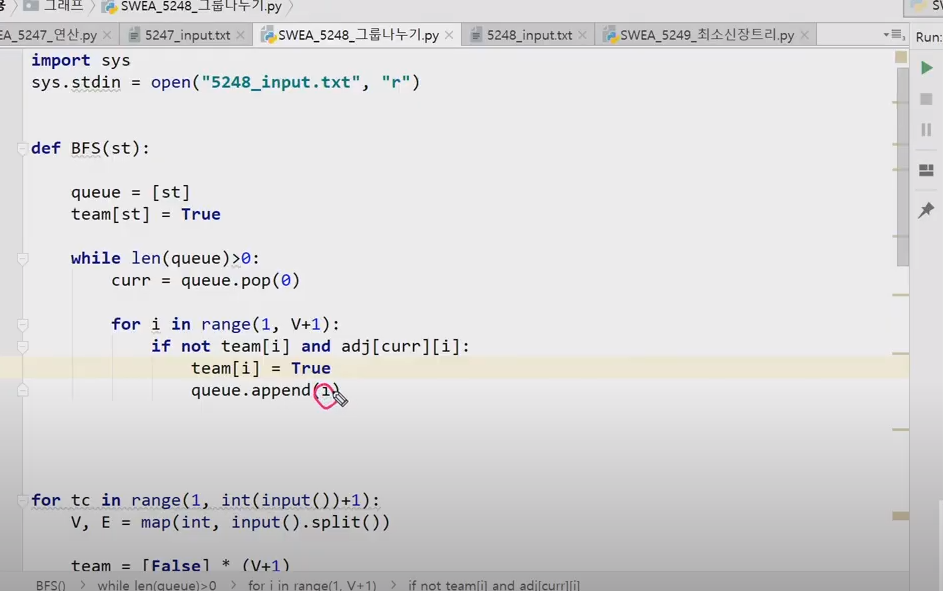
# BFS
- How it works
- Current Location : V
- One stack needed for TF visited. Second stacked needed to record visited order.
- One queue needed to keep track of order to visit
- starting point set as V
- enQueue V to queue
- enQueue childern
- deQueue and move to children
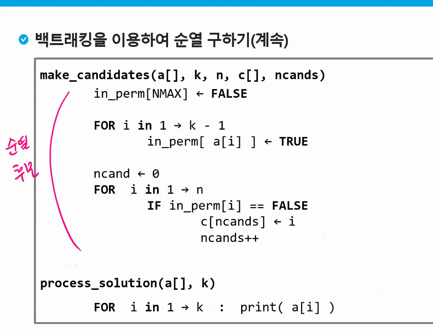
# Backtracking
Meaning
- When you cannot find the answer in a certain branch, you 'backtrack' to a different branch to find the right answer.
- Optimization problems
- Decision problems : Is there an answer? ex:Maze, n-Queen, map coloring, subset sum
How it works - Maze
- Two stacks needed : visited true false stack and last visited push/pop stack
- Push every coordinates you visited to push/pop stack as well as marking True on true false stack.
- When you hit a dead end, pop from push/pop stack one by one. You will backtrack one coordinate at a time.
- This is basically DFS, but at every node you check whether it is 'promising'
- If it is not 'promising', you backtrack to its' parent node and DFS again.
How it works - N Queen
- You want to place N number of queens on a chess board.
- Place the first queen on the first row, first column
- Second queen must be placed on a second row, but some cells are already pruned. By default place the second queen on the available first left column. (Note that in a DFS case, we would place queens on all possible scenarios AND THEN confirm whether it is viable or not)
- Carry on until you cannot place queen on the next row OR you placed N number of queens and reached solution
- If you reached a dead end, you backtrack to prior rows and place queens on the next option.
- Continue until you placed N number of queens
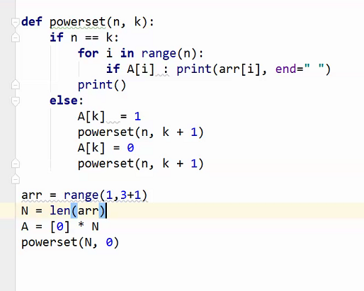
How it works - Power Set
- Powerset meaning : All subsets including itself and empty set
- Number of powerset is always $2^n$
- Method : Use list with N number of True/False items.
- Powerset is the set of all subsets of different sizes!
- Any subset can be represented as a bit string of length N.
- First build a list of.
B=[0]*len(set). This will be used to generate bitstrings. - Second make list of bitstrings. This will save all possible bitstrings.
bitstrings=[] - Generate Bitstrings.
generateBitstrings(0, B, bitstrings)
def generateBitstrings(i, B, bitstrings):
	if i == N:
		bitstrings.append(B.deepcopy())
	else :
		#Divided to two cases each time. The B list which is [0, 0, 0, ... 0]
		# ith item is changed to either 1 or 0 everytime. When recursion reaches i==N,
		# Every item has been modified and then added to list bitstrings.
		B[i] = 1
		generateBitstrings(i+1, B, bitstrings)
		B[i] = 0
		generateBitstrings(i+1, B, bitstrings)
1
2
3
4
5
6
7
8
9
10
11- Use bitstrings to select items.
subsets = []
for bitstring in bitstrings:
	subset = []
	for i in range (len(set)):
		bit = bitstring[i]
		if bit ==1:
			subset.append(set[i])
	subsets.append(subset)
return subsets
1
2
3
4
5
6
7
8
9Backtracking vs DFS
- Backtracking involves a method called 'Pruning'
- By 'pruning' not 'promising' 'nodes' early on, you don't have to search every possible case.
- Generally backtracking is faster than DFS